Examples
Running the inversions in the examples folder is the best and easiest way to learn how to use Bayesian1DEM. Each follows the standard inversion workflow.
Step1: Initialize
This should be the only script you have to write from scratch for each data set. Because it is unique to each inversion, this script is stored in the examples folder. It script should create three structures—S, S1, and S2—that contain the data, metadata, and inversion parameters described under Inputs. These structures must then be saved to separate files. In the examples, these are given the names <FileName>.mat, WaterColumn.mat, and Subsurface.mat, but you can name them whatever you want.
Creating this script can be tricky, so use the Step1 scripts in the examples folder as templates for creating your own.
Step2: Run Inversion
Like the rest of the steps, this script is stored in the “CommandScripts” folder. It simply calls the function PT_RJMCMC, which is the main inversion workhorse. This is the step that might take a long time to run, depending on the total number of iterations you requested and the cost of each forward evaluation. Each step costs one forward evaluation, which is typically the most expensive part of the algorithm, so you should be able to estimate how long it should take to run. But the algorithm estimates the completion time every S.displayEvery steps.
The only input arguments PT_RJMCMC needs are the names of the files where the input structures are saved and where to write the output (the model ensemble). The output files are of the form <FileName>_PT_RJMCMC_#.mat, where “#” is the chain number in terms of the parallel tempering temperature ladder (from high temperature to low, such that the highest numbers correspond to the lowest temperaturess).
Step3: Assess Convergence
This script takes as input the file name where the S structure is saved and the number of parallel tempering chains you ran in Step2 and produces a series of plots assessing the convergence of the algorithm to the posterior distribution.
Assessing convergence of MCMC algorithms is not easy, and it’s fairly subjective. The plot in the upper-left shows RMS as a function of iteration; in the upper-right is a plot showing the number of layer interfaces as a function of iteration. In the center are the acceptance rates of the various perturbation moves (birth, death, move interface, update). In the lower-left is the swap rate of the parallel tempering chains; and in the lower-right is a plot of RMS misfit for each data type in case of jointly inverting multiple data sets. The main thing to look for when assessing convergence is stationarity: there should be some jitter to all of the curves (Bayesian inversion is inherently stochastic), but you want to make sure they go “flat” at a certain point. Before that point is considered “burn-in” and is discarded (not considered part of the model ensemble).
The main point of Step3 is to assess whether Bayesian1DEM converged or not, and to determine the burn-in.
Step4: Combine Chains
In case you ran multiple chains at T = 1, this script takes each of the T = 1 Markov chains, removes the burn-in, and combines the rest into the posterior model ensemble, which it saves in the file <FileName>_PT_RJMCMC_Combined.mat. This script also chooses 50 models at random from the model ensemble, generates modeled data for each, and plots the model responses alongside the data for each data type you inverted. As such, this script requires you to indicate all the data types included in the inversion. You also must specify the burn-in, the number of Markov chains, and the number of chains at T = 1. The script will also make a histogram of RMS misfit across all models in the ensemble.
Step5: Plot Posterior
This script makes plots of marginal probability density as a function of depth and resistivity; Kullback-Leibler divergence (for assessing data sensitivity to the model parameters as a function of depth); the distribution of probability density for interfaces; and a histogram of the number of layer interfaces.
Other than the name of the file where the structure S is stored, this script requires that you provide three parameters:
thin — decimation of the model ensemble. Make this larger if this step is taking a long time to run. Adjacent models in the ensemble are highly similar to one another anyway, so decimation (up to a point) shouldn’t affect the output of this script by much.
G.dz, G.drho — the posterior PDFs produced by this script are binned; G.dz determines the size of the depth bins, while G.drho determines the size of the resistivity bins. Making these smaller slows this script down considerably.
Example 1: joint inversion of MT and surface-towed CSEM field data
These data were collected offshore New Jersey and first published in Gustafson et al (2019) [Gustafson19]. These data were also inverted using Bayesian1DEM (see Blatter et al, 2019 [Blatter19]). Funding for the collection of this data was provided by National Science Foundation grants 1458392 and 1459035.
The first step is to run the script “Running Step1_Initialize_Freshwater_Inversion.m”. This should produce the following output files
Trash/Line1_Joint_ST121-135_MT3.mat
Trash/WaterColumn.mat
Trash/Subsurface.mat
as well as the following plots of the MT and CSEM data
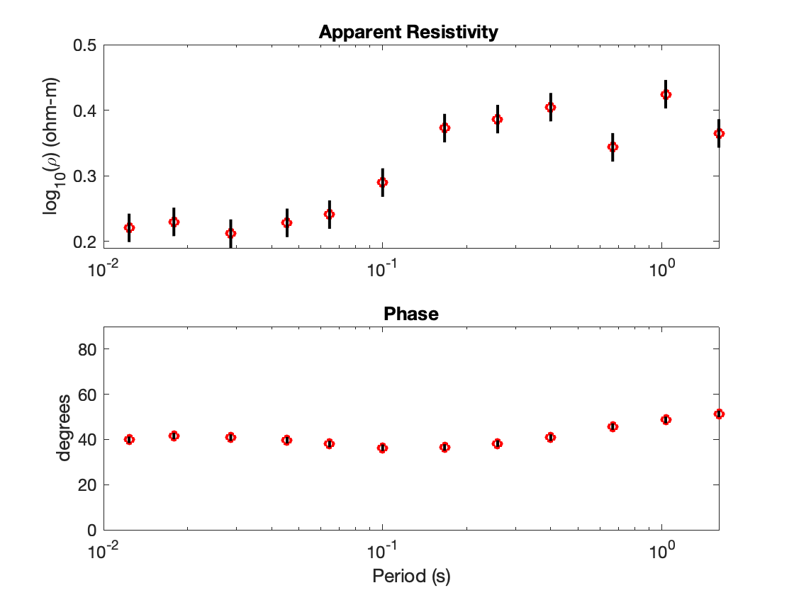
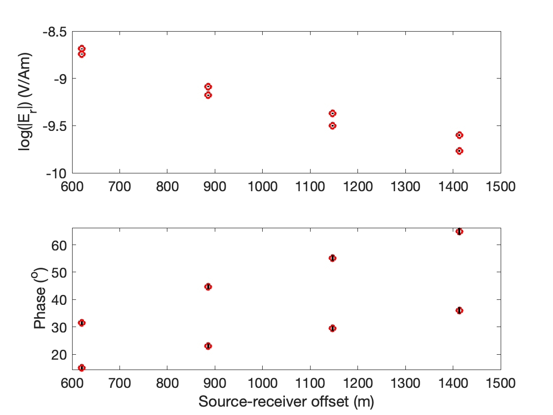
To run the inversion, simply run Step2_runBayesianInversion.m; but before you do, uncomment the line “FileNameRoot = ‘Line1_Joint_ST121-135_MT3’;” while making sure that the other lines are commented out. Updated information about the RMS of the current model, the mean time per iteration, and the expected completion time should be printed to the command window every few seconds (unless you changed S.displayEvery). Depending on your computer, this inversion should take about 30 minutes to run. To keep the run time short enough for this example to be a learning tool, the total number of iterations was kept low (50,000). In reality, to properly converge S.numIterations should probably be set to at least 200,000 or more. When Bayesian1DEM has finished running, the command window will display the message “At last, done with PT_RJ_MCMC. Proceed to Step 3.”
Next, run “Step3_assessConvergence.m” after making sure the line “FileNameRoot = ‘Line1_Joint_ST121-135_MT3’;” is uncommented while the rest of those lines are commented out. Two figures should pop up, one each for regions 1 and 2. The one for region 2 (the subsurface) is the one on top, where the y-axis of the plot in the upper-right corner goes from 0-40 (not 1-7). This figure is shown below
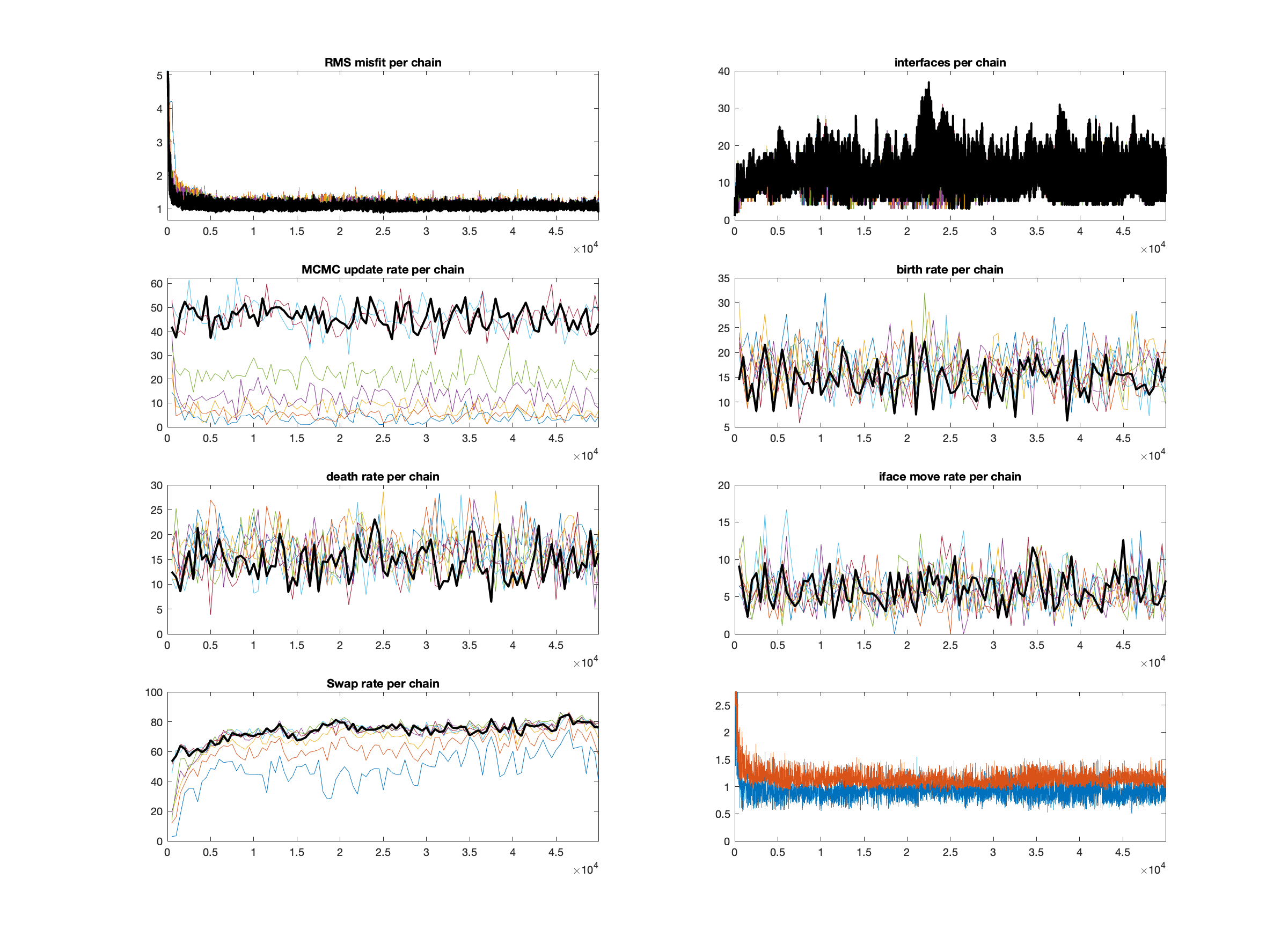
All the plots in this figure should become fairly stationary after iteration 10,000-20,000 or so, indicating that this is the burn-in phase (iterations 1-20,000). The acceptance rates (depending on the type of perturbation) should all be between 5-50% or so. Note that the number of interfaces rarely if ever reaches the maximum allowed (40); this is a good sign that the data are not demanding more model complexity than we are allowing the models to have. The parallel tempering chain swap rates should be between 20-80% or so, indicating good mixing and sharing of models between the chains. In the lower-right, both the red and blue curves are stationary and fitting the data well, indicating that the models are satisfying both MT and CSEM data sets, rather than just one or the other. Overall, these are healthy convergence statistics. Ideally, I would run this inversion for much longer than 50,000 steps, but even so these chains will provide a halfway decent estimate of the posterior distribution.
To run Step 4, first do the following. In Step4_combineChains.m,
As before, uncomment “FileNameRoot = ‘Line1_Joint_ST121-135_MT3’;” and comment the rest.
Change the burn-in to a number in the range 10,000-20,000, depending on how your Step 3 plots look.
Set MT and stCSEM equal to 1, and set DRC and obCSEM to 0.
This script should produce the following three figures
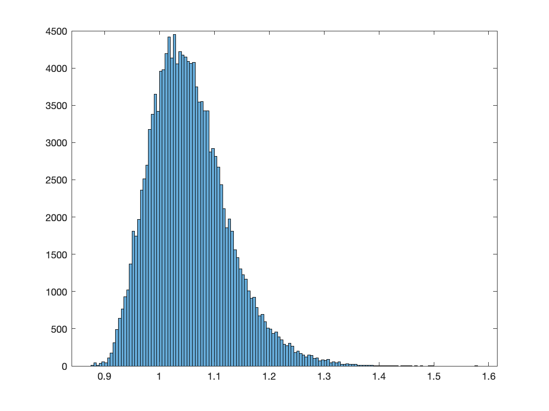
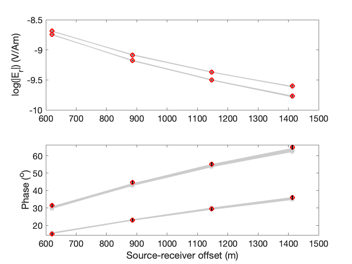
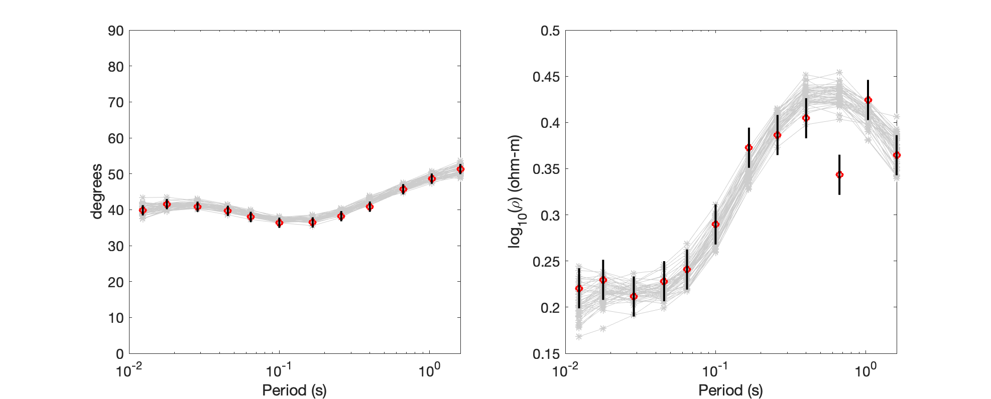
The first is a histogram of (combined) RMS misfit across all the models in the ensemble (the post burn-in models in all three T = 1 Markov chains). This should show a range of misfits distributed in the range 0.9-1.4 or so. This indicates we are fitting the data well in an aggregate sense. To see if we are fitting each data set and all data points well, the other two figures show the data along with the model responses of 50 randomly selected models from the ensemble in gray. While some data are clearly noisy, these plots should show that the models in the ensemble are fitting all the data adequately.
This script has produced an output file, “Line1_Joint_ST121-135_MT3_PT_RJMCMC_Combined.mat” which, in addition to having one heck of a file name, contains the entire model ensemble (as defined above). If you want to extract specific statistical information about the inverted model parameters, this is the collection of models to use to do that.
Speaking of which, let’s run Step 5: Step5_plotPosterior.m. Other than the usual commenting/uncommenting of the file name, set both G.dz and G.drho to 0.05 or so then run the script! It should take just a few seconds to run, producing the following figure
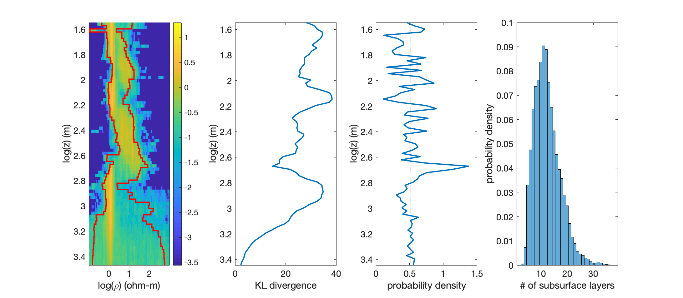
The first plot on the left is the main course: our estimate of the posterior distribution of probability density as a function of depth and resistivity. At each depth, this plot contains a marginal distribution, meaning the probability sums to one from left to right across the plot at each depth. The warmer colors indicate regions of higher probability density while the cooler colors indicate the opposite. The left and right red lines represent the 5th and 95th percentiles, respectively, at each depth. The region between them is known as the 90% credible interval and indicates the range of resistivity spanned by 90% of the models in the ensemble.
In the center-left panel is a plot of the Kullback-Leibler divergence (See [Blatter19] for details). The gist of it is that the KL divergence reflects the information content of the data — basically, by how much the data have changed our prior assumptions that all resistivities and interface locations are equally likely. Where the KL divergence is high, the data are contributing a lot to our understanding of the subsurface; where it is low, the data are not informative. Note that the KL divergence tapers to 0 at the bottom of the model space (2,500 m depth and deeper), indicating that Bayesian1DEM isn’t needing to place interfaces deeper than we are allowing it to (the data have lost sensitivity by the time we reach the bottom of the model domain).
In the center-right panel is a plot of interface probability. There’s a lot of scatter in this plot except around 2.7 log units, where a large spike indicates a high probability of an interface at this depth. the jitter in these three plots will quite likely decline if Bayesian1DEM is run for longer (250,000 steps, say).
Finally, the plot on the far right is a histogram of the number of interfaces across all models in the ensemble. Note that while we are letting the data choose the number of model parameters needed to fit the data (up to a max of 40 interfaces), most models have around 10 interfaces only. This is a good example of “Bayesian parsimony”, which means that, all else being equal, Bayesian inversion algorithms prefer models with fewer parameters (not the fewest—fewer).
And we’re done! Again, if you have specific research questions, design your own scripts to mine the model ensemble (“Line1_Joint_ST121-135_MT3_PT_RJMCMC_Combined.mat”) for relevant statistics to help you answer those questions. You’ve generated the model ensemble at no insignificant computational cost—use it to the max!
The other examples run in the same way. Use the Step 1 scripts as templates to help you design your own for inverting your data. Good luck!